Classification Metrics for Score Histograms

In a previous post, Metrics for Calibrated Classifiers, a method was provided to compute confusion matrix statistics and derived metrics, based on only a distribution of scores produced by a well calibrated classifier. It was noted that:

since the confusion matrix estimates can be determined at any threshold, curves like precision-recall curves and ROC curves can be determined parametrically as can metrics derived from these curves.

This post expands on the previous ideas and provides a method for computing confusion matrix statistics for histograms of scores (for instance, provided in python via numpy.histogram). The motivation for providing a histogram based method is to reduce the memory constraints over the method outlined in the original article.

Example

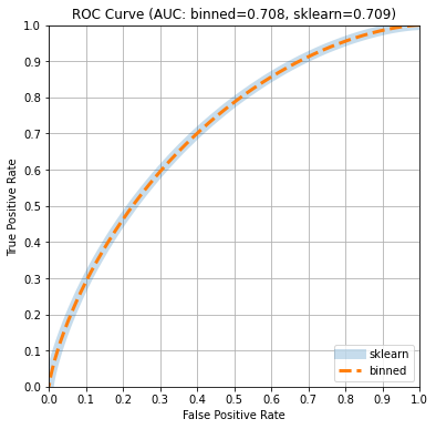
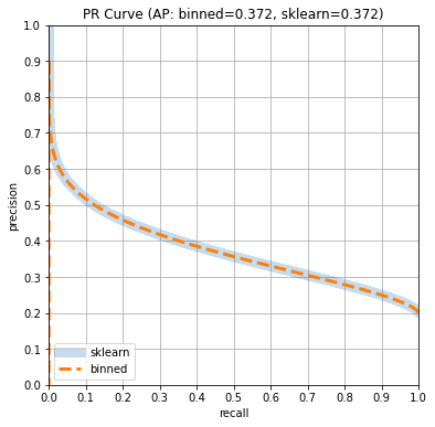
We will compare the ROC and PR curve and the AUC and AP estimates computed by scikit-learn with curves estimated without any ground truth (yt) information. While ground truth information is omitted from the calculations, the information is provided implicitly if the classifier from which the predictions are derived is well calibrated. This means that the accuracy of a positive prediction equals the probability output by the classifier.

Create a sample distribution

Create a Beta(α=2, β=8) distribution representing probability estimates and sample 10 million ground truth labels (yt) and predictions (yp).

Use scikit-learn to determine ROC curve and PR curves

Here, scikit-learn returns AUC: 0.709 AP: 0.372 and takes about 14 seconds on a modern MacBook Air. If we produce the precision recall curve and ROC curve, we see the following.

Compute the confusion matrix stats based on predictions only

We can determine the confusion matrix stats established for a histogram with a constant bin width.

This only takes about 1 second to compute.

Plot ROC and PR curves

ROC Curve	PR Curve

`plot_roc(cm,sk_fpr,sk_tpr,sk_auc)`	`plot_pr(cm,sk_rec,sk_pre,sk_ap)`

Conclusion

Since the “classifier” represented by the Beta distribution is well calibrated, the curves computed by scikit-learn, which use the predictions and ground truth, are aligned with the estimates computed by the method in this post that do not require the ground truth. Consequently, the area under the curves is also nicely aligned. We can plot these curves or compute the areas under the curves based only on histograms of probabilities. For large scale analysis, score histograms can be computed in parallel and reduced to avoid an explosion of memory and the results are similar in quality to the method provided in Metrics for Calibrated Classifiers with much lower memory overhead. While the example in this post only used the Beta distribution, the reader is encouraged to try other distributions and other parameter settings like digits_precision in cm_stats_by_threshold_binned to see how the method degrades.