Metrics for Calibrated Classifiers
Introduction
We can model a calibrated classifier as a random variable \(Y\), whose support is a subset of \(\left[ 0, 1 \right]\). Accordingly, if we denote the probability density function as \(f_{Y}\) and the cumulative distribution function as \(F_{Y}\), then given a threshold, \(t\), we can define the expected confusion matrix as:
| predicted cond / true cond |
true | false |
|---|---|---|
| true | TP: \(\int_{t}^{1} y f_{Y}(y) dy\) | FP: \(1 - F_{Y}(t) - \int_{t}^{1} y f_{Y}(y) dy\) |
| false | FN: \(\int_{0}^{t} y f_{Y}(y) dy\) | TN: \(F_{Y}(t) - \int_{0}^{t} y f_{Y}(y) dy\) |
Given these values, we can compute any desired metric one might find in the Precision and recall Wikipedia article.
Derivation
It should be easy to see and follows from the definitions that the following are true:
\[N = FN + TN = F_{Y}(t) \\ P = TP + FP = 1 - F_{Y}(t) \\ N + P = 1\]If we think about the definition of \(TP\), it is the expected value of scores that exceed the threshold, \(t\), or:
\[TP = \int_{t}^{1} y f_{Y}(y) dy\]Note that the upper integration limit of one comes from the fact that the support for \(Y\) is upper bounded by one since calibrated classifiers output probabilities. \(FP\) is simply \(P - TP\).
\(FN\) is defined similarly to \(TP\), since it is an estimate of true values that are less than \(t\):
\[FN = \int_{0}^{t} y f_{Y}(y) dy\]The only differences are the integration limits. Note the lower integration limit follows from the fact that calibrated classifiers output probabilities (which must be non-negative). \(TN = N - FN\).
Metrics based on a sample of scores
Given a sample of scores generated by a calibrated classifier, we can use the confusion matrix formulae above by linearly scanning the scores and accumulating the sum and count of scores that exceed and do not exceed the threshold.
| variable | definition |
|---|---|
| \(TP\) | sum of scores that exceed the threshold |
| \(P\) | count of scores that exceed the threshold |
| \(FN\) | sum of scores that do not exceed the threshold |
| \(N\) | count of scores that do not exceed the threshold |
| \(FP\) | \(P - TP\) |
| \(TN\) | \(N - FN\) |
If desired, each of these can be divided by the sample size to ensure that:
\[TP + FP + FN + TN = 1\]this will make \(TP\) and \(FN\) true positive and false negative rates. It will also make \(P\) and \(N\) related to the CDF, but this normalization will not have an effect on computing any of the metrics based on ratios of combinations of \(TP\), \(FP\), \(FN\) and \(TN\).
Experiments
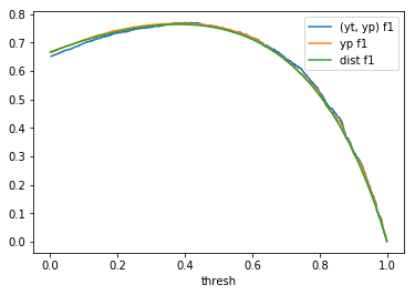
To illustrate the ability to estimate classification metrics for a calibrated classifier, we devise the following series of experiments. Let \(\mathcal{ D }\) be a probability distribution representing a calibrated classifier (i.e., with support in \([0, 1]\)). Sample \(n\) random variates from \(\mathcal{D}\) and for each variate, \(p_i\), perform a weighted coin flip with positive probability \(p_i\). These weighted coin flips are draws from \(Bernoulli(p_i)\) distributions. Define \(yp \in \mathbb{R}^n\) as the probabilities drawn from \(\mathcal{ D }\) and \(yt \in \{0, 1\}^n\) as the associated Boolean values drawn from \(Bernoulli(p_i)\).
To compute the (yt, yp) column in table 1, we use \(yt\) and \(yp\) and determine the metrics using
\(yp\) as the threshold (i.e., the decision boundary) values. These metrics are computed using the *_score
methods from scikit-learn’s sklearn.metrics module. The yp column in table 1 is
computed using the methodology outlined in the Metrics based on a sample of scores section above.
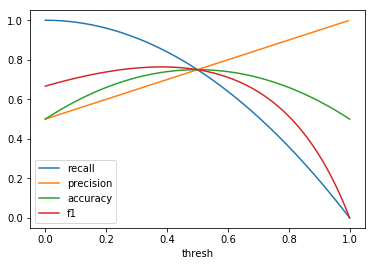
Finally, the dist column is determined by applying the desired metrics to the confusion matrix values computed
with the formulae in the introduction. In table 1, this process is repeated for several distributions
with \(n = 2000\).
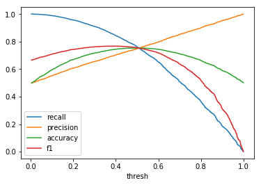
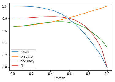
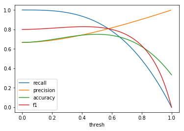
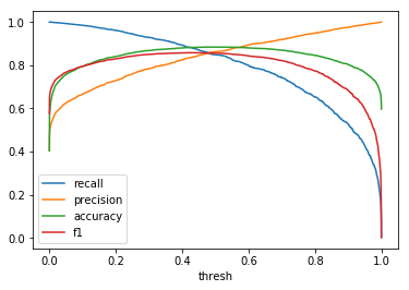
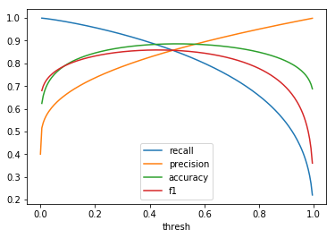
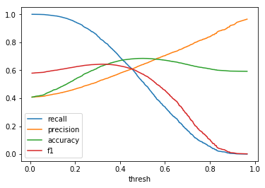
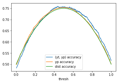
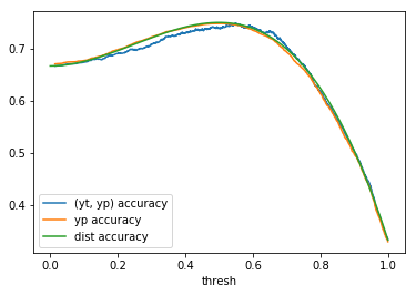
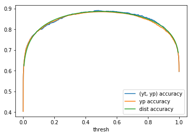
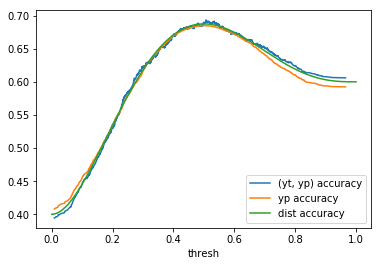
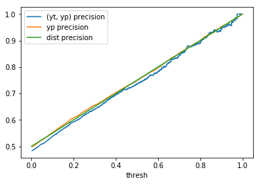
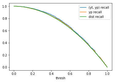
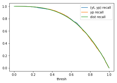
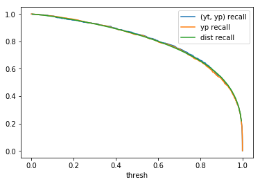
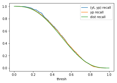
Table 1: By distribution and calculation method
| (yt, yp) | yp | dist | |
|---|---|---|---|
| \(U(0, 1)\) | 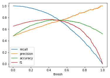 |
 |
 |
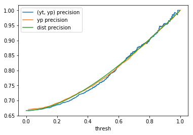
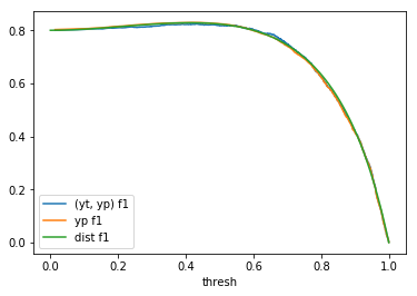
| \(F(x) = x^2\) | 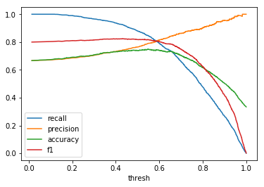 |
 |
 |
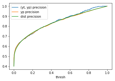
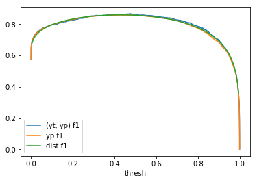
| \(Beta(0.2, 0.3)\) | 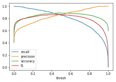 |
 |
 |
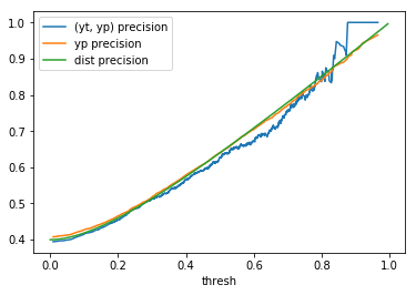
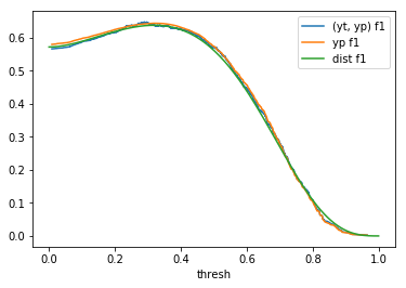
| \(Beta(2, 3)\) | 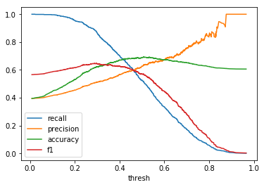 |
 |
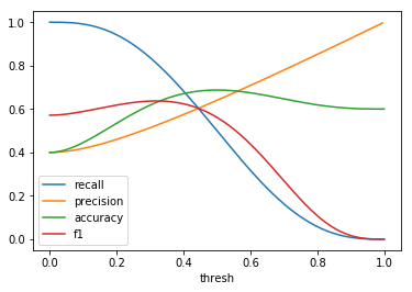 |
Table 2: By distribution and metric
| U(0, 1) | F(x) = x2 | β(0.2, 0.3) | β(2, 3) |
|---|---|---|---|
 |
 |
 |
 |
 |
 |
 |
 |
 |
 |
 |
 |
 |
 |
 |
 |
Discussion
When comparing plots for each distribution in table 1, notice the yp plots are smoother than the (yt, yp) plots and the dist plots are smoother than the yp plots. Metrics based only on yp can be thought of like metrics in (yt, yp) except that \({c_i \to \infty}\), rather than 1, coin flips are drawn from each \(Bernoulli(p_i)\). The dist metrics can be thought of like the metrics based on yp as \({n \to \infty}\).
Also note that metric values based on yp seem to approach the dist metric values. It seems that this convergence is predicted to occur with high probability according to the Glivenko–Cantelli theorem (1933).
One additional point: since the confusion matrix estimates can be determined at any threshold, curves like precision-recall curves and ROC curves can be determined parametrically as can metrics derived from these curves.
Conclusion
If you have reason to believe that a classifier is calibrated (e.g., it was explicitly calibrated), then classification metrics can be directly computed from the classifier’s scores without the need for ground truth data. While this may not be a perfect solution, it provides a good back-of-the-napkin estimate. If the distribution is known, the classification metrics can be computed analytically from the distribution’s CDF and expectations over the intervals \([0, t)\) and \([t, 1]\).