An Optimally Efficient Online Estimate of the Number of Matched Entities with Successes

Given a set of matches with success probabilities:

one might want to estimate the number of elements in \(A\), \(B\), or \(A \cup B\) that are involved in a successful match. Done naïvely, this involves calculating an expectation that is as complex to calculate as calculating the PMF of the Poisson binomial distribution. We can sum \(\text{ops}(n,k)\), from the previous post Poisson binomial distribution, over \(k=0,1,\dots ,n\) to get:

where we add in the multiplication operations necessary to calculate the expectation. This shows that when calculated naïvely, it would take an exponential amount of operations to calculate the number of entities with a success.

Example 1

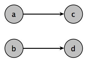
Let’s say that we are doing biparitite matching and we’ve produced the following matches:

Then we can determine the number of entities expected to see at least one success with the following formula:

The probabilities (on the right) should be familiar to those who’ve seen the Poisson binomial distribution. The coefficients \(\left\{ 0, 2, 2, 4 \right\}\) need some explaining. In this example, we’re ascribing the successful events, when they occur, to both entities involved in the match. The coefficient is the number of unique entities that appear in success probability subscripts of each term or addend. For instance, in the first line, there are no success probabilities—only failure probabilities—so the coefficient is \(0\).
\(b\) and \(d\) occur in the second term so the coefficient is 2; \(a\) and \(c\) occur in the third term so the coefficient is 2; \(a\), \(d\), \(c\) and \(d\) occur in the fourth term so the coefficient is 4. The expectation, once simplified is \(2 p_{ac} + 2 p_{bd}\).

Example 2

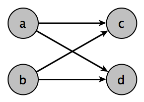
This example has the following matches:

and the expectation calculation, as calculated in the previous example, becomes:

which simplifies to:

This calculation, while accurate requires exponential runtime and it also requires an understanding of the topology of graph to determine the coefficients.

A Better Way

When thinking about what we’re trying to accomplish, it should be pretty clear that we are trying to determine the expectation of the number of entities in at least one successful match. The probability of an entity being involved in at least one successful match is one minus the probability of being involved in zero successful matches. So, if for an entity, \(a\), we aggregate the matches involving \(a\), we can write the probability of \(a\) being in at least one successful match as:

where \(M_{a}\) is the set of matches involving \(a\). Then if we want to calculate the distribution of the number entities involved in at least one successful match, the appropriate distribution is the Poisson binomial distribution. The expectation of the Poisson binomial distribution is just the sum of the success probabilities that parameterize the distribution. See the wikipedia page for details. So, if we want to calculate the expectation, we take the sum of the probabilities of the entity being in at least one successful match. This is just:

It may not be immediately obvious but this algorithm is \(O(N)\) where \(N\) is the number of matches. Here’s the algorithm:

Algorithm 1

1. Create a hash map with entity IDs for keys and a linked list of probabilities for each match involving the entity ID in the associated map key.
2. For each match: \(\left(i, j, p_{ij} \right)\), place \(p_{ij}\) in the list associated with key \(i\) (Optionally, place \(p_{ij}\) in the list associated with key \(j\), if the match is ascribed to both entities).
3. For each key-value pair in the map, calculate the probability of at least one successful match using equation 1.
4. Sum the resultant probabilities.

Since we only ever iterate over the match probabilities twice, and hash map and linked list insertion and iteration is \(O(1)\) per operation, the algorithm is \(O(N)\).

Equivalence

simplifies to \(2 p_{ac} + 2 p_{bd}\). AND

simplifies to

These are the same as the expectations from the naïve calculation.

Algorithm 2

One might notice that the linked lists in Algorithm 1 are overkill and completely unnecessary. Instead we can do the following:

1. Create a hash map, \(M\) with entity IDs in \(\mathbb{N}\) for keys and values in \(\mathbb{R}\). The starting value, for each associated key, should be 1.
2. For each match: \(\left(i, j, p_{ij} \right)\)
3. \(\quad \left(i, v\right) \leftarrow \left(i, v \left(1 - p_{ij}\right) \right)\)  
4. \(\quad \left(j, v\right) \leftarrow \left(j, v \left(1 - p_{ij}\right) \right)\) (Optionally, if match is ascribed to both entities).
5. Compute the sum of \(1 - v, \forall v \in M\).

Algorithm 2 Code

1
2
3
4
5
6
7
8
9
10
11
12
13
14
// Scala Code
case class Match(i: Int, j: Int, prob: Double)

def entitiesWithASuccessfulMatch(matches: TraversableOnce[Match], 
                                 ascribeSuccessToBoth: Boolean): Double = {
  matches.foldLeft(Map.empty[Int, Double]){(ps, m) => 
    val si = ps.getOrElse(m.i, 1d) * (1 - m.prob)
    if (ascribeSuccessToBoth) {
      val sj = ps.getOrElse(m.j, 1d) * (1 - m.prob)
      ps ++ List(m.i -> si, m.j -> sj)
    }
    else ps + (m.i -> si)
  }.valuesIterator.foldLeft(0d)((s, x) => s + 1 - x)
}

Algorithm 2 Remarks

One very special property to note here is that the input to entitiesWithASuccessfulMatch is a TraversableOnce, which, as should be obvious by the name, can only be traversed once. Since we don’t copy matches to a data structure that can be traversed multiple times, this algorithm is an online algorithm. If we think of the matches as a graph, then this algorithm takes \(O(E)\) time and \(O(V)\) auxiliary space.

What’s even cooler is that with a very small amount of work, we can turn this algorithm into a monoid. This allows the algorithm to be trivially parallelized.

Monoid Code

1
2
3
4
5
6
7
8
9
10
11
12
13
14
15
16
17
18
19
20
21
22
23
24
25
26
27
28
29
30
31
32
33
34
35
36
37
38
39
40
41
42
43
44
45
46
47
48
49
50
51
52
53
// Scala Code
trait Monoid[A] {
  def append(a: A, b: A): A
  def zero: A
}

case class Match(i: Int, j: Int, prob: Double)

case class SuccessCounter private(ps: Map[Int, Double]) {
  /**
   * @return expectation of the number of entities involved in a 
   *         successful match.
   */
  def expectation = ps.valuesIterator.foldLeft(0d)((s, x) => s + 1 - x)
  
  /**
   * Convenience plus method that delegates to the monoid.
   * @param e2
   */
  def +(e2: SuccessCounter) = SuccessCounter.monoid.append(this, e2) 
}

object SuccessCounter {
  def apply(matches: TraversableOnce[Match], 
            ascribeSuccessToBoth: Boolean): SuccessCounter = {
            
    val pss = matches.foldLeft(Map.empty[Int, Double]){(ps, m) => 
      val si = ps.getOrElse(m.i, 1d) * (1 - m.prob)
      if (ascribeSuccessToBoth) {
        val sj = ps.getOrElse(m.j, 1d) * (1 - m.prob)
        ps ++ List(m.i -> si, m.j -> sj)
      }
      else ps + (m.i -> si)
    }
    
    SuccessCounter(pss)
  }

  implicit object monoid extends Monoid[SuccessCounter] {
    def append(e1: SuccessCounter, 
               e2: SuccessCounter) = {
      val (small, large) = if (e1.ps.size < e2.ps.size) 
                             (e1.ps, e2.ps) 
                           else (e2.ps, e1.ps)
      val m = small.foldLeft(large){ case (lrg, (k, p)) => 
        lrg + (k -> lrg.getOrElse(k, 1d) * p) 
      }
      SuccessCounter(m)
    }
  
    def zero() = SuccessCounter(Map.empty)  
  }
}

Monoid Calling Code Example

1
2
3
4
5
6
7
8
9
10
11
12
val e1 = SuccessCounter(Seq(Match(1, 3, 1d/2), Match(1, 4, 1d/3)), true)
val e2 = SuccessCounter(Seq(Match(2, 3, 1d/5), Match(2, 4, 1d/7)), true)
val e3 = e1 + e2

// 2.009523809523809 = 211/105
e3.expectation

val e4 = SuccessCounter(Seq(Match(1, 3, 1d/2), Match(1, 4, 1d/3),
                            Match(2, 3, 1d/5), Match(2, 4, 1d/7)), true)

// 2.009523809523809 = 211/105
e4.expectation

Remarks

There’s something really satisfying about this algorithm, not only because of the linear rather than exponential runtime, but also because it doesn’t keep track of the graph topology. This not only makes the algorithm much faster, but it’s much simpler conceptually.

We’ve shown that this algorithm is both an online algorithm meaning we can update the results as data becomes available, and a monoid, so we can easily parallelize the algorithm.