Poisson Binomial Revisited
Since I wrote on the Poisson Binomial Distribution, I was bothered by a couple of things. The first and main problem that I had was with stack overflows and excessive \(O\left( { n }^{ 2 } \right)\) memory allocation in method 2. As a reminder method 2 found in (Chen and Liu, 1997) looks like:
\[R\left( k,C \right) =R\left( k, C \backslash \{ k \} \right) +{ w }_{ k }R\left( k-1, C \backslash \{ k \} \right)\]This may or may not look like gibberish to those who haven’t read the paper but I find Table 1 from the paper to be quite informative.
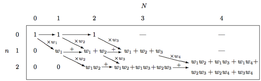
This diagram also drove me crazy until I had the epiphany that allowed me to rewrite method 2 non-recursively using only \(O\left( n \right)\) space rather than \(O\left( { n }^{ 2 } \right)\) auxiliary space. The epiphany was this.
Epiphany
The diagram, when interpreted as a matrix, is a matrix in row echelon form. These zeros on the left are worthless to the algorithm and if we remove them and appropriately shift the remaining values to the left, the diagonal arrows in the diagram become vertical, downward arrows. This doesn’t affect the left-to-right arrows but this gives us a diagram that looks like a triangle. The fact that we have only downward and right arrows and a triangular shape helps a lot. It indicates that we can iterate over the rows then columns and use just a one-dimensional array, \(r\), of size \(n + 1\) to aggregate the computation because we only need values from the previous iteration of the outer loop and the previous value of the current inner loop to update the current value in the inner loop. Once the algorithm completes this array will contain the PMF. This means that we can use bottom-up dynamic programming to generate the PMF for the Poisson binomial distribution. At the end of each iteration of the inner loop, we add another value toward the end of the array that represents the probability of a certain number of successes, where the probability of zero successes is the last value in the array, the probability of one success is the second to last value, and so on. The only gotcha is that we need to normalize each value by multiplying by the normalizing constant from equation 5 in the paper:
\[\prod _{ i\in S }{ { \left( 1+{ w }_{ i } \right) }^{ -1 } }\]Finally, we just have to reverse the array, \(r\).
Benefits
There are multiple benefits to writing the algorithm this way:
- Stack overflows don’t occur.
- Memory consumption is greatly reduced from \(O\left( { n }^{ 2 } \right)\) to \(O\left( n \right)\) and the \(O\left( n \right)\) memory allocation is necessary to hold the PMF.
- The actual speed of the algorithm is faster (wall clock, not asymptotic runtime).
Code
1
2
3
4
5
6
7
8
9
10
11
12
13
14
15
16
17
18
19
20
21
22
23
24
25
26
27
28
29
30
31
32
33
34
35
36
37
38
39
40
41
42
43
44
45
46
47
48
49
50
51
52
53
54
55
56
57
58
59
60
61
62
63
64
65
66
67
68
69
70
71
72
73
74
75
76
77
78
79
80
81
82
// Scala Code

object PoissonBinomial {
  val zero = BigDecimal(0)
  val one = BigDecimal(1)

  def pmf(pr: TraversableOnce[Double]): Array[BigDecimal] = pmf(pr, Int.MaxValue, 2)

  def pmf(pr: TraversableOnce[Double], maxN: Int, maxCumPr: Double): Array[BigDecimal] = {
    require(0 <= maxN)

    // This auxiliary array, w, isn't necessary for the algorithm to
    // work correctly but memoization saves redundant computation.
    // Since we are using it, we can base all subsequent computation
    // on w and make pr a TraversableOnce.
    val w = pr.map{p =>
      val x = BigDecimal(p)
      x / (1 - x)
    }.toIndexedSeq
    val n = w.size
    val mN = math.min(maxN, n)
    val z = w.foldLeft(one)((s, w) => s / (w + one))
    val r = Array.fill(n + 1)(one)

    r(n) = z

    var i = 1
    var j = 0
    var k = 0
    var m = 0
    var s = zero
    var cumPr = r(n)

    while(cumPr < maxCumPr && i <= mN) {
      s = zero;  j = 0;  m = n - i;  k = i - 1

      while (j <= m) {
        s += r(j) * w(k + j)
        r(j) = s
        j += 1
      }

      r(j - 1) *= z
      cumPr += r(j - 1)

      i += 1
    }

    finalizeR(r, i, n)
  }

  def finalizeR(r: Array[BigDecimal], i: Int, n: Int) = {
    if (i <= n) {
      val smallerR = new Array[BigDecimal](i)
      System.arraycopy(r, n - i + 1, smallerR, 0, i)
      reverse(smallerR)
    }
    else reverse(r)
  }

  def reverse[A](a: Array[A]): Array[A] = {
    val n = a.length / 2
    var i = 0
    var t = a(0)
    var j = 0
    while (i <= n) {
      j = a.length - i - 1
      t = a(i)
      a(i) = a(j)
      a(j) = t
      i += 1
    }
    a
  }
}

def time[A](a : => A) = {
  val t1 = System.nanoTime
  val r = a
  val t2 = System.nanoTime
  (r, (1.0e-9*(t2 - t1)).toFloat)
}
Remarks
This code doesn’t read like typical Scala code because it uses mutable arrays and while
loops rather than functional constructs like folds.
The purpose was speed and correctness over conciseness and elegance. This choice stems from the pmf algorithm’s
runtime and space requirements: \(O\left( { n }^{ 2 } \right)\) and \(O\left( n \right)\), respectively.
The memory that is allocated contains the PMF are the end of the algorithm. Thus, no auxiliary space is necessary and the algorithm is optimally space efficient.
Another comment. The runtime for computing the full PMF is
indeed \(O\left( { n }^{ 2 } \right)\), but if we just want to know the probabilities for the first \(k\) successes,
the runtime is more like \(O\left( k n \right)\). This is nice since the code was written to short circuit if the
caller only requests the first \(k\) probabilities. The code can also short circuit for using it as an
inverse distribution function
by specifying maxCumPr. The length - 1 of the resulting array is the IDF value.
Tests
On my 2010 MacBook Pro, I can run val p = PoissonBinomial.pmf(Seq.fill(1000)(0.5)) in about 0.5 seconds and
it’s accurate according to Wolfram Alpha. p(500) is 0.02522501817836080190684168876210234 and Wolfram Alpha
says it’s 0.025225. p(1000) is
9.332636185032188789900895447238125E-302 and Wolfram Alpha says it’s
9.33264×10^-302.
What’s more important is that the algorithm based on BigDecimal can handle large probabilities whereas
an implementation based on 64-bit IEEE 754 floats will eventually
numerically overflow given a large enough set of probabilities. Avoiding this obviously comes at a cost. The cost is
unfortunately both in terms of speed and memory. Because large probabilities make the normalizing constant small
when there are a lot of probabilities in the computation, the BigDecimal values need to add a lot of precision and
this is where the speed slowdowns and increased memory usage come in. So the runtime actually depends somewhat on
the probability value inputs. This is OK because when the number of probabilities is small (< 1000), the runtime is
reasonable (on the order of a few seconds). But when opting for an exact algorithm over an approximation, correctness
should always trump speed. If this is not acceptable, thanks to the
Central limit theorem,
one can always use a (refined) normal approximation
(see Poisson Binomial Distribution).
License
The above code is released under the MIT License, Copyright (c) 2016 Ryan Deak.
References
- Chen, Sean X., and Jun S. Liu. “Statistical applications of the Poisson-binomial and conditional Bernoulli distributions.” Statistica Sinica 7.4 (1997): 875-892.